1. Interpretation. SUR, CSV and EB
The Ratio of Variation (RV) is the quotient between the highest and the lowest standardised rate across the units of study. It is a simple and intuitive way to determine how large the variation is; for example, a RV of 2 would represent a 2-fold difference between the area with the highest rate and the area with the lowest rate.
With some frequency, areas under study have very few cases, even no cases in a determined time-span. In this case, the ratio would reach unusually high values likely associated to random noise. To reduce the risk of misinterpreting RV in these extreme situations, usually affecting those countries with very small areas, ECHO calculates systematically the ratio between the rates in the 5th and 95th percentiles - noted as RV95-5. Along the same idea of getting stable numbers, ECHO also reports the ratio in the centre of the distribution of rates, variation that is not supposed to be affected by random phenomena, noted as ratio in the interquartile ratio (IQR or RV75-25).
In spite of its simplicity and extremely intuitive interpretation, RV is too sensitive to areas with few cases and/or extreme values. This forces to interpret RV in the context of the rest of statis-tics, particularly those including the effect of chance in their formulation.
ECHO usually estimates three statistics that deal with true (systematic) variation – variation beyond random noise: a) the Standardised Utilisation Ratio (SUR); b) the Systematic Component of Variation (CSV); and, c) Empirical Bayes Statistic (EB). The three statistics take as a reference the expected variation, for the specific phenomenon and the population under analysis.
a) Standardised Utilisation Ratio (SUR)
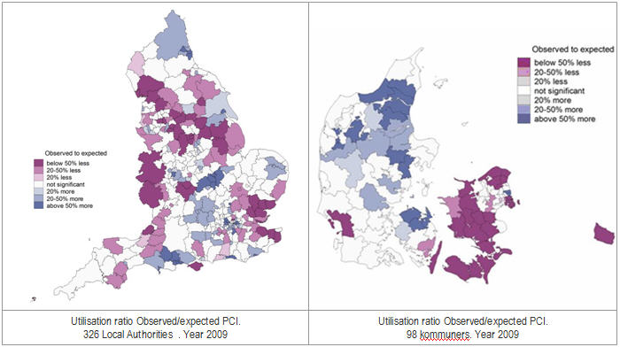
SUR is the quotient between observed to expected cases in a healthcare area. The expected cases are derived from the age-sex specific risk of the event of study in the standard population – areas of a particular country in the in-country analyses, or all ECHO areas in cross-country comparisons.
Expected cases are derived from: ei = ∑j, knijk Rjk, where nijk is the population in area i, age group j and sex stratum k, and Rjk is the age-sex specific risk for the whole region under study. Hence, the quotient of the observed to the expected number of cases is the indirect Standardised Utilisation Ratio, SURi = yi/ei for the i-th Healthcare Area. This quotient is in fact the maximum-likelihood estimator of ri, the unknown relative risk of suffering a given surgical procedure in the area, under the assumption that yi ~Poisson(eiri) independently for each i-th Health Area.
Close technical note
Interpretation:
An area with SUR equals 1 would mean that its behaviour is similar to the “average” pattern of utilisation. As any other ratio, its values can move in two directions: from 1 to infinite repre-senting utilisation above the “average” pattern; and from 0 to 1, representing utilisation below the “average” pattern.
While values above 1 are interpreted straightforwardly, a SUR of 1.8 represents a risk of expo-sure an 80% higher than the “average pattern”, in those values below 1, it is first required to calculate the inverse of SUR; thus, a value of 0.8 would represent a 25% (1 divided by 0.8) less exposure than the “average” pattern.
b) Systematic Component of Variation (CSV) and, c) Empirical Bayes Statistic (EB).
Although SUR overcomes the simplicity of the RV in measuring the magnitude of variation, signaling areas statistically different to the null value (i.e. risk equals 1), the estimations are still affected by extreme values.
SCV and EB, although less intuitive, are also able to differentiate systematic and random variation while reducing the effect of extreme values.
SCV and the EB statistics are derived under a more general framework where the number of admissions per area is modeled hierarchically in a two-step procedure. The first step assumes that, conditional on the risk ri, the number of counts yi follows a Poisson distribution, yi|ri ~Poisson(eiri), whereas in the second one, heterogeneity in rates is modeled adopting a common distribution π for the risk ri (or for its logarithm), ri~ π(r|θ), with θ the vector of parameters of the density function. Whereas the derivation of the SCV does not require a parametric form for π, as the SCV is precisely the moment estimator of the variance in the distribution of π, the EB statistics is based on the assumption that the log-relative risks are normally and identically distributed, log(ri) ~N(μ, σ2). Estimates for the parameters such as the variance component σ2 and predictions for the random effects representing ri, EB are derived from a Penalized Quasi Likelihood method.
Close technical note
Interpretation:
Values different from zero are to be interpreted as systematic differences across areas and conversely, a value of zero points to homogeneous behaviour across the territory. In other words, high SCV or EB values would then suggest that a significant part of the observed variation could not be deemed random.
How much variation? The answer is not a clear-cut issue. The more the value of SCV or EB, the more likely the variation is systematic; however, given that there is not a prescriptive value in assessing the variation, empirical calibrators can be of use to establish the relative importance of the variation detected. So, the SCV or EB value in the procedure of interest is compared with the SCV or EB value in a calibrator, a condition o procedure that usually stands for the lowest variation. This strategy has been largely used taking as a calibrator hip fracture repair. ECHO utilizes different calibrators, depending on the subject of study: hip fracture, AMI admissions, colectomy in colorectal cancer, hysterectomy in uterus cancer, etc.
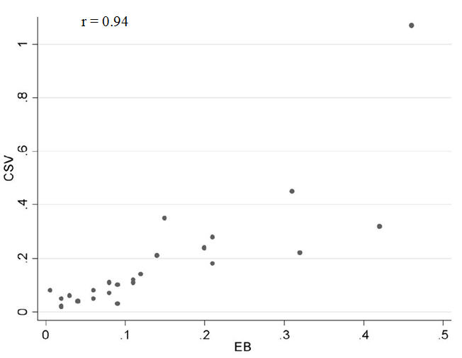
The correlation between both statistics is very high – the figure represents the correlation in several procedures and conditions with different basal rate and variation. However, EB tends to be more robust with small numbers and actually, as seen in the graph, is more conservative than CSV – EB values are closer to the null value 0.
Correlation between CSV an EB values
![]() Note: In ECHO, when the goal is on analysing an individual country the standard population is the population of the country under study; however when international comparison is the goal, the standard population is built using all the ECHO countries.
Note: In ECHO, when the goal is on analysing an individual country the standard population is the population of the country under study; however when international comparison is the goal, the standard population is built using all the ECHO countries. 


